Building Electricity Networks#
The preparation process of the PyPSA-Eur energy system model consists of a group of snakemake
rules which are briefly outlined and explained in detail in the sections below.
Not all data dependencies are shipped with the git repository.
Instead we provide separate data bundles which can be obtained
using the retrieve* rules (Retrieving Data).
Having downloaded the necessary data,
build_shapesgenerates GeoJSON files with shapes of the countries, exclusive economic zones and NUTS3 areas.build_cutoutprepares smaller weather data portions from ERA5 for cutouteurope-2013-era5and SARAH for cutouteurope-2013-sarah.
With these and the externally extracted ENTSO-E online map topology
(data/entsoegridkit), it can build a base PyPSA network with the following rules:
base_networkbuilds and stores the base network with all buses, HVAC lines and HVDC links, whilebuild_bus_regionsdetermines Voronoi cells for all substations.
Then the process continues by calculating conventional power plant capacities, potentials, and per-unit availability time series for variable renewable energy carriers and hydro power plants with the following rules:
build_powerplantsfor today’s thermal power plant capacities using powerplantmatching allocating these to the closest substation for each powerplant,build_natura_rasterfor rasterising NATURA2000 natural protection areas,build_ship_rasterfor building shipping traffic density,build_renewable_profilesfor the hourly capacity factors and installation potentials constrained by land-use in each substation’s Voronoi cell for PV, onshore and offshore wind, andbuild_hydro_profilefor the hourly per-unit hydro power availability time series.
The central rule add_electricity then ties all the different data inputs
together into a detailed PyPSA network stored in networks/elec.nc.
Rule build_bus_regions#
Creates Voronoi shapes for each bus representing both onshore and offshore regions.
Relevant Settings#
countries:
See also
Documentation of the configuration file config/config.yaml at
Top-level configuration
Inputs#
resources/country_shapes.geojson: confer Rule build_shapesresources/offshore_shapes.geojson: confer Rule build_shapesnetworks/base.nc: confer Rule base_network
Outputs#
resources/regions_onshore.geojson: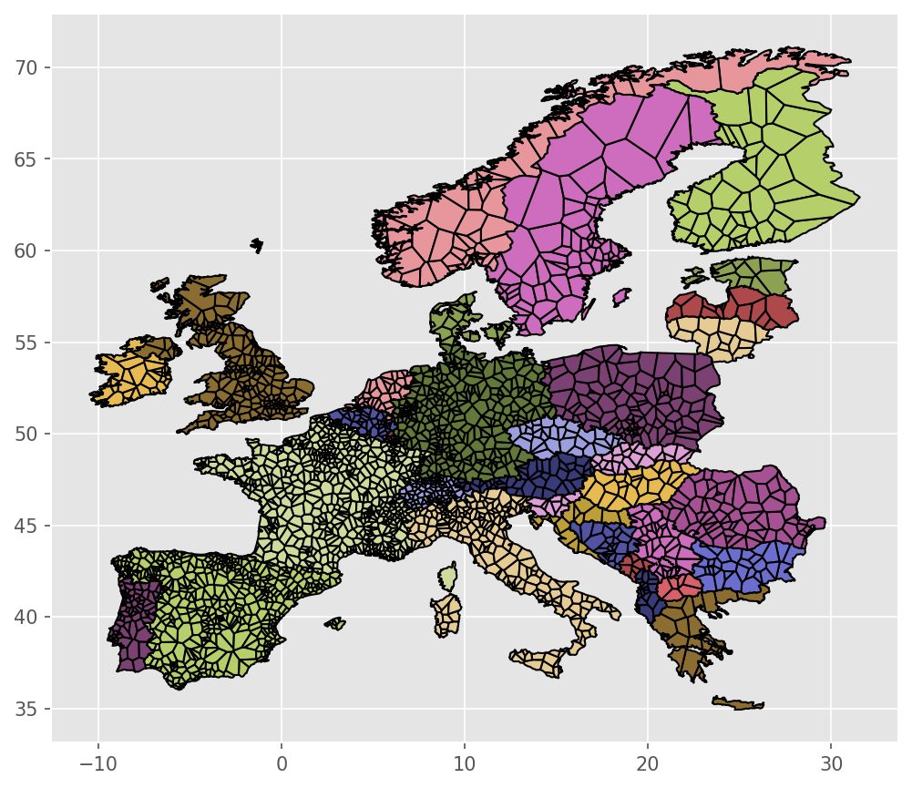
resources/regions_offshore.geojson: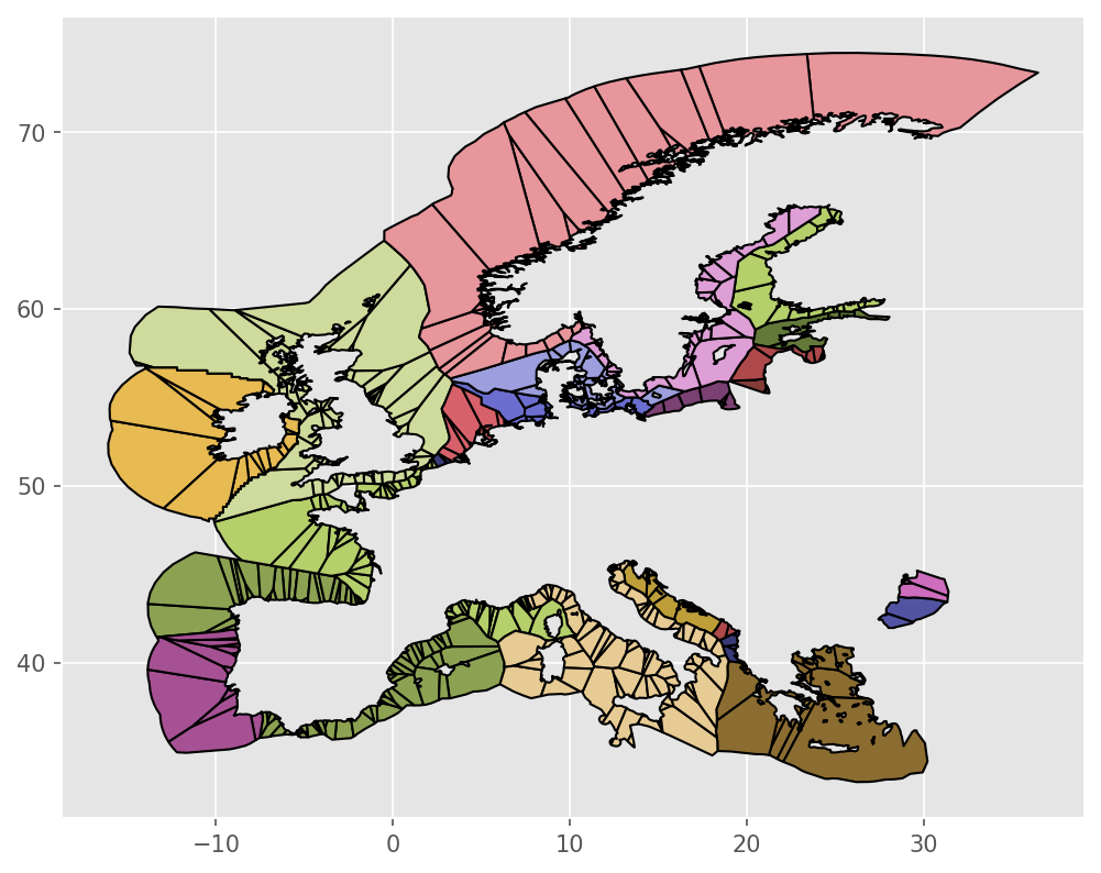
Description#
Rule build_cutout#
Create cutouts with atlite.
For this rule to work you must have
installed the Copernicus Climate Data Store
cdsapipackage (install with `pip`) andregistered and setup your CDS API key as described on their website.
See also
For details on the weather data read the atlite documentation. If you need help specifically for creating cutouts the corresponding section in the atlite documentation should be helpful.
Relevant Settings#
atlite:
    nprocesses:
    cutouts:
        {cutout}:
See also
Documentation of the configuration file config/config.yaml at
atlite
Inputs#
None
Outputs#
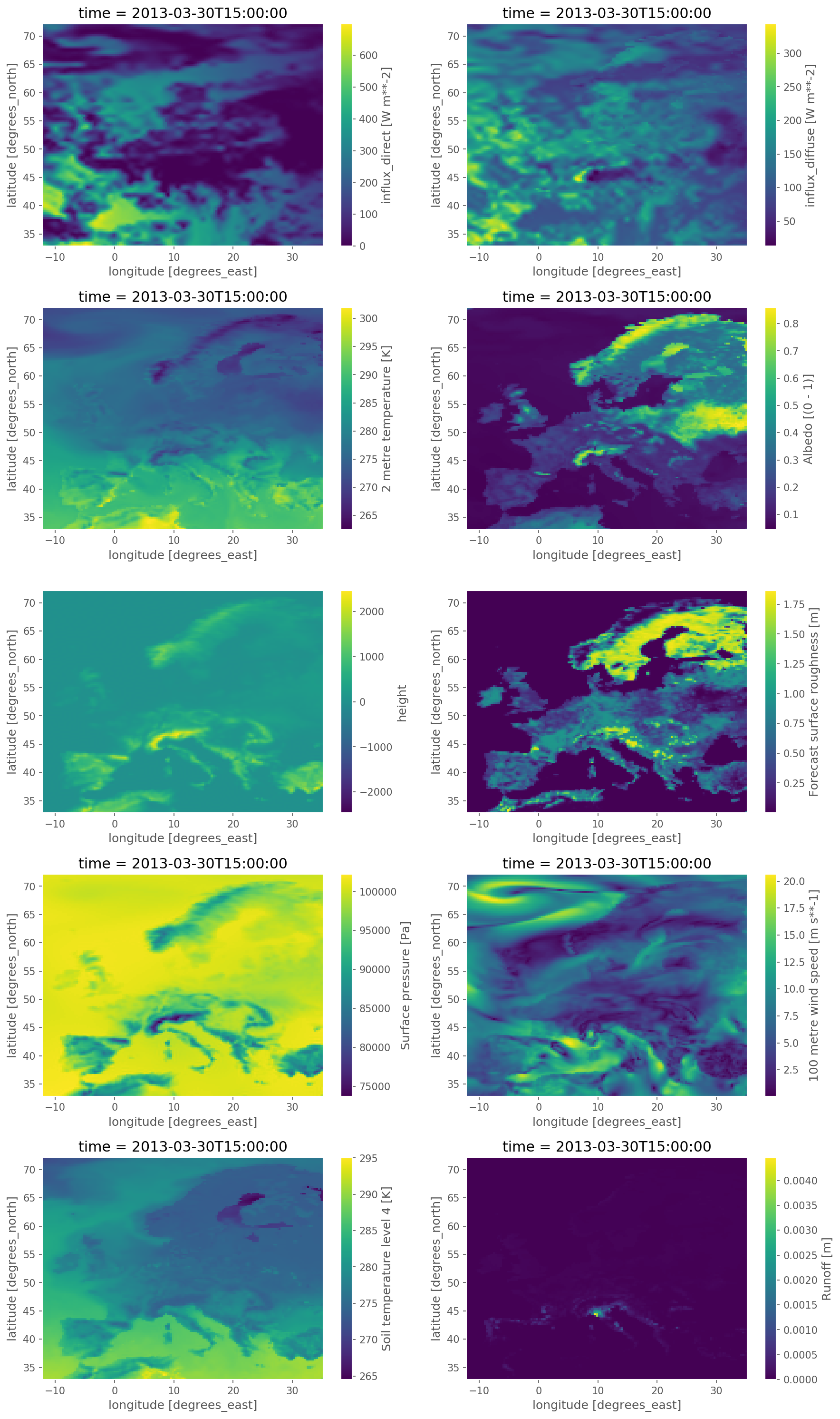
cutouts/{cutout}: weather data from either the ERA5 reanalysis weather dataset or SARAH-2 satellite-based historic weather data with the following structure:
ERA5 cutout:
Field
Dimensions
Unit
Description
pressure
time, y, x
Pa
Surface pressure
temperature
time, y, x
K
Air temperature 2 meters above the surface.
soil temperature
time, y, x
K
Soil temperature between 1 meters and 3 meters depth (layer 4).
influx_toa
time, y, x
Wm**-2
Top of Earth’s atmosphere TOA incident solar radiation
influx_direct
time, y, x
Wm**-2
Total sky direct solar radiation at surface
runoff
time, y, x
m
Runoff (volume per area)
roughness
y, x
m
Forecast surface roughness (roughness length)
height
y, x
m
Surface elevation above sea level
albedo
time, y, x
–
Albedo measure of diffuse reflection of solar radiation. Calculated from relation between surface solar radiation downwards (Jm**-2) and surface net solar radiation (Jm**-2). Takes values between 0 and 1.
influx_diffuse
time, y, x
Wm**-2
Diffuse solar radiation at surface. Surface solar radiation downwards minus direct solar radiation.
wnd100m
time, y, x
ms**-1
Wind speeds at 100 meters (regardless of direction)
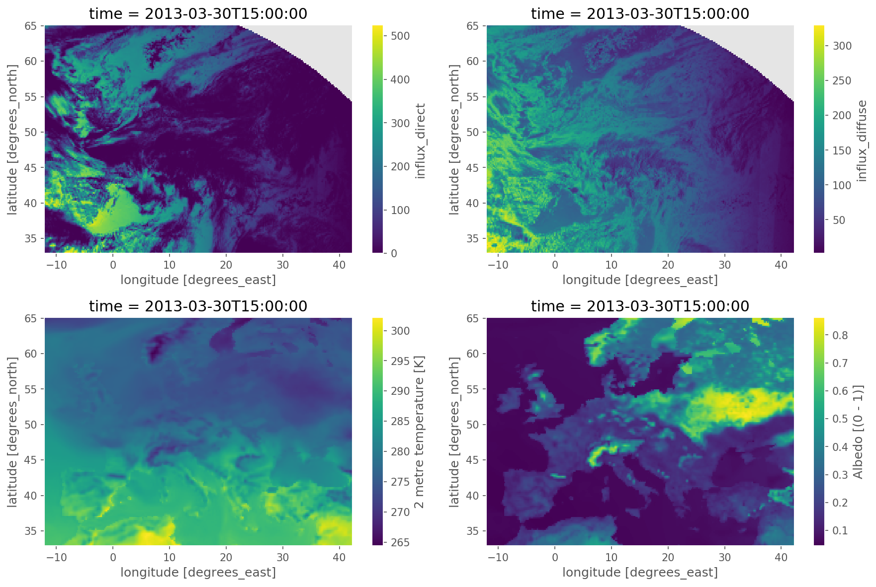
A SARAH-2 cutout can be used to amend the fields temperature, influx_toa, influx_direct, albedo,
influx_diffuse of ERA5 using satellite-based radiation observations.
Description#
Rule prepare_links_p_nom#
Extracts capacities of HVDC links from `Wikipedia.
<https://en.wikipedia.org/wiki/List_of_HVDC_projects>`_.
Relevant Settings#
enable:
    prepare_links_p_nom:
See also
Documentation of the configuration file config/config.yaml at
Top-level configuration
Inputs#
None
Outputs#
data/links_p_nom.csv: A plain download of https://en.wikipedia.org/wiki/List_of_HVDC_projects#Europe plus extracted coordinates.
Description#
None
Rule build_natura_raster#
Rasters the vector data of the `Natura 2000.
<https://en.wikipedia.org/wiki/Natura_2000>`_ natural protection areas onto all cutout regions.
Relevant Settings#
renewable:
    {technology}:
        cutout:
See also
Documentation of the configuration file config/config.yaml at
renewable
Inputs#
data/bundle/natura/Natura2000_end2015.shp: Natura 2000 natural protection areas.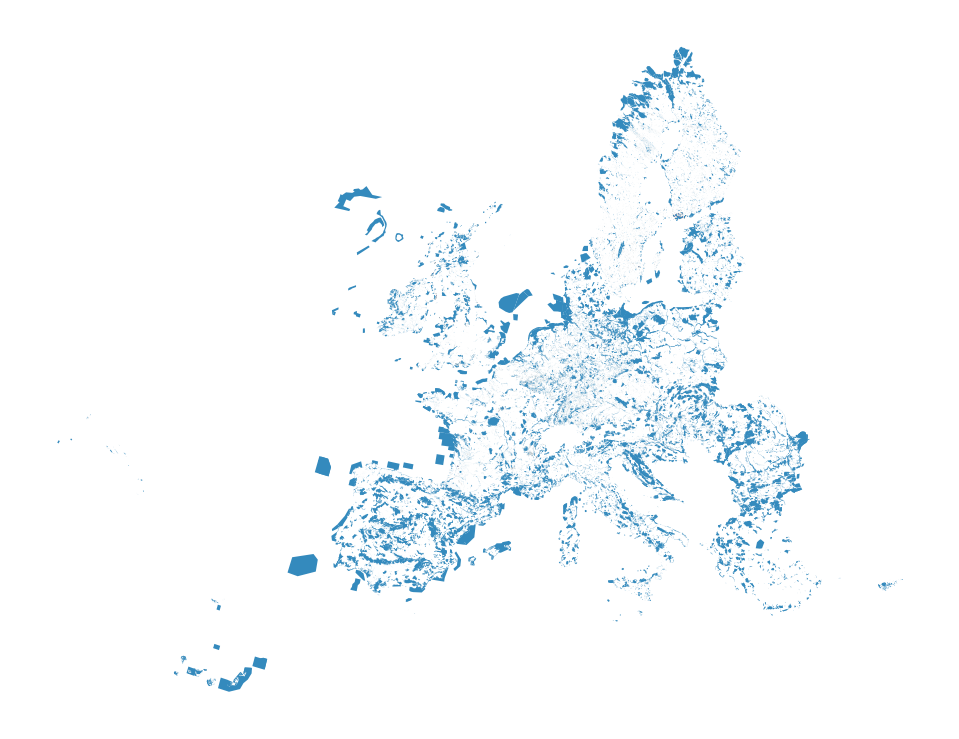
Outputs#
resources/natura.tiff: Rasterized version of Natura 2000 natural protection areas to reduce computation times.
Description#
Rule base_network#
Creates the network topology from a `ENTSO-E map extract.
<PyPSA/GridKit>`_ (March 2022) as a PyPSA network.
Relevant Settings#
countries:

electricity:
    voltages:

lines:
    types:
    s_max_pu:
    under_construction:

links:
    p_max_pu:
    under_construction:
    include_tyndp:

transformers:
    x:
    s_nom:
    type:
See also
Documentation of the configuration file config/config.yaml at
snapshots, Top-level configuration, electricity, load,
conventional, links, transformers
Inputs#
data/entsoegridkit: Extract from the geographical vector data of the online ENTSO-E Interactive Map by the GridKit toolkit dating back to March 2022.data/parameter_corrections.yaml: Corrections fordata/entsoegridkitdata/links_p_nom.csv: confer linksdata/links_tyndp.csv: List of projects in the TYNDP 2018 that are at least in permitting with fields for start- and endpoint (names and coordinates), length, capacity, construction status, and project reference ID.resources/country_shapes.geojson: confer Rule build_shapesresources/offshore_shapes.geojson: confer Rule build_shapesresources/europe_shape.geojson: confer Rule build_shapes
Outputs#
networks/base.nc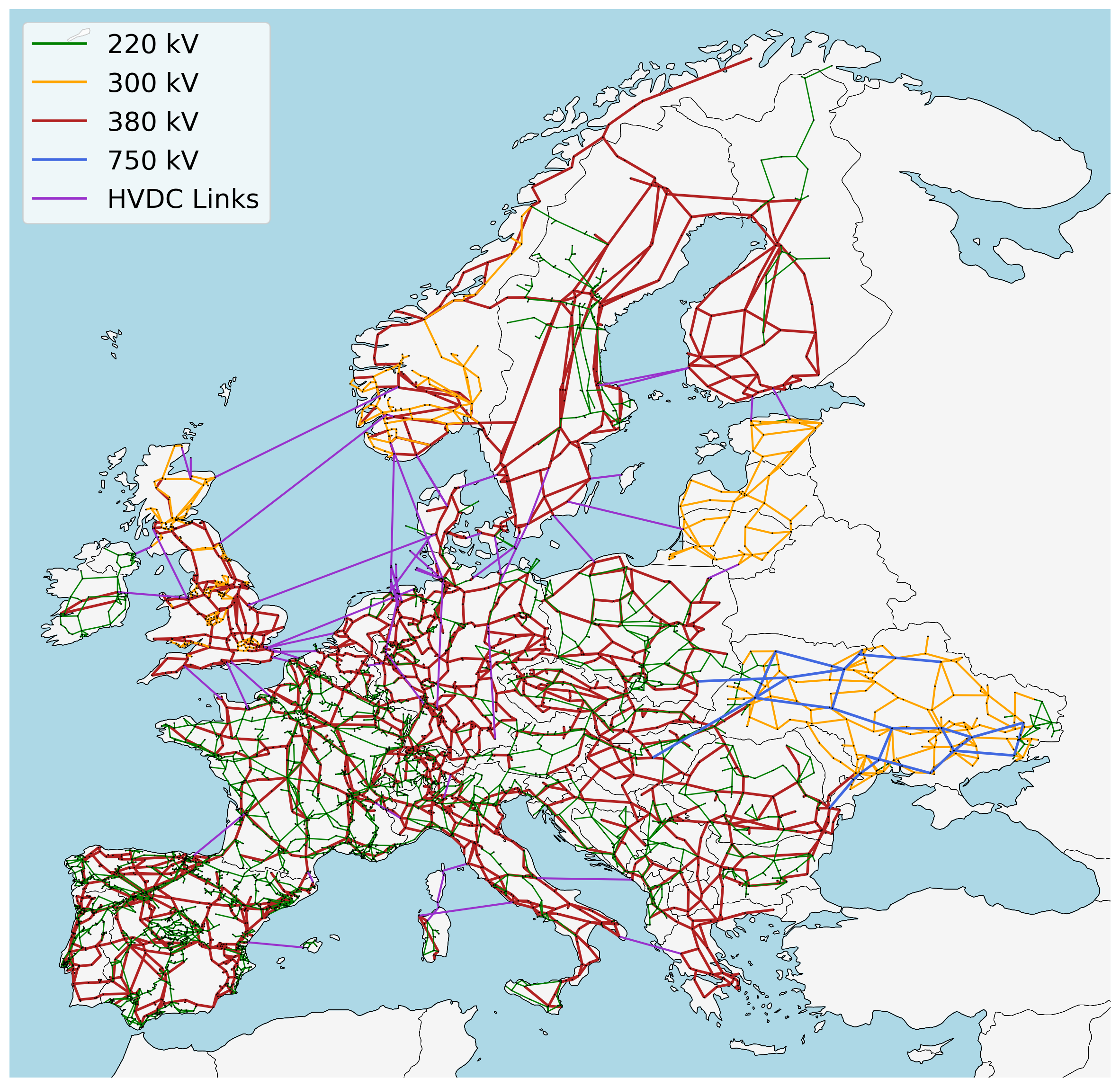
Description#
Rule build_shapes#
Creates GIS shape files of the countries, exclusive economic zones and `NUTS3 < https://en.wikipedia.org/wiki/Nomenclature_of_Territorial_Units_for_Statistics> `_ areas.
Relevant Settings#
countries:
See also
Documentation of the configuration file config/config.yaml at
Top-level configuration
Inputs#
data/bundle/naturalearth/ne_10m_admin_0_countries.shp: World country shapes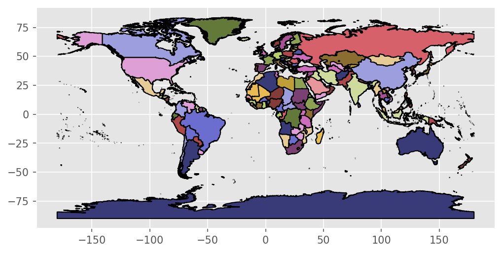
data/bundle/eez/World_EEZ_v8_2014.shp: World exclusive economic zones (EEZ)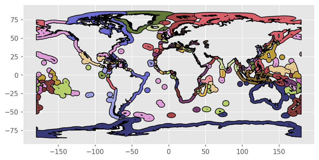
data/bundle/NUTS_2013_60M_SH/data/NUTS_RG_60M_2013.shp: Europe NUTS3 regions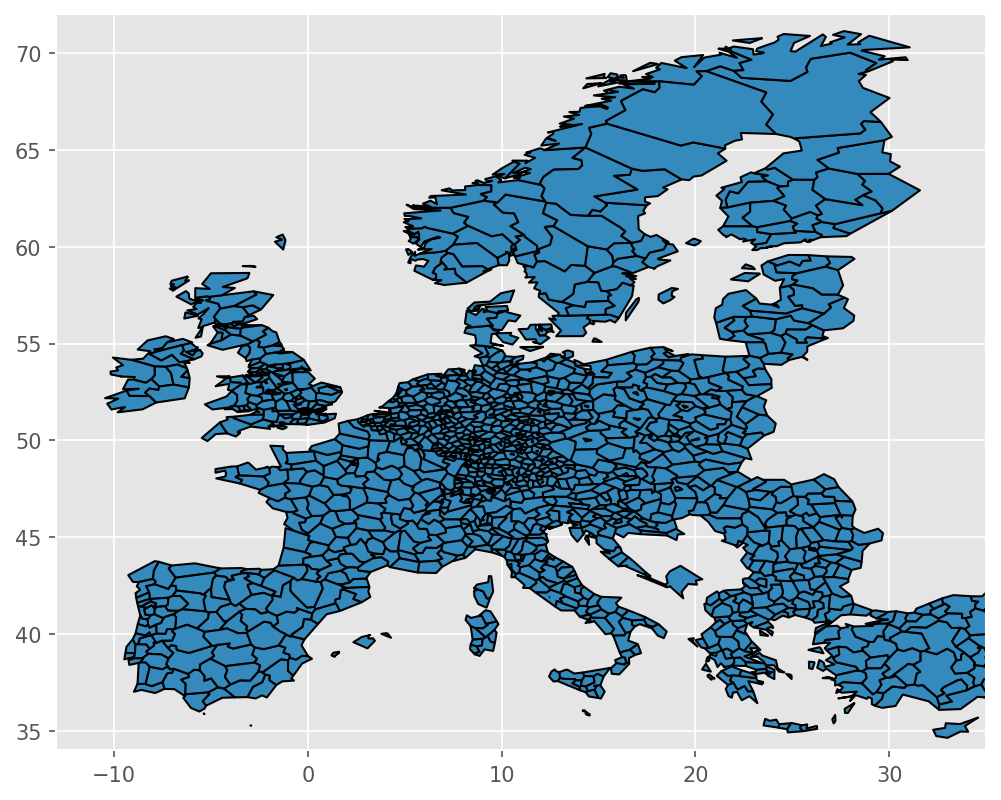
data/bundle/nama_10r_3popgdp.tsv.gz: Average annual population by NUTS3 region (eurostat)data/bundle/nama_10r_3gdp.tsv.gz: Gross domestic product (GDP) by NUTS 3 regions (eurostat)data/bundle/ch_cantons.csv: Mapping between Swiss Cantons and NUTS3 regionsdata/bundle/je-e-21.03.02.xls: Population and GDP data per Canton (BFS - Swiss Federal Statistical Office )
Outputs#
resources/country_shapes.geojson: country shapes out of country selection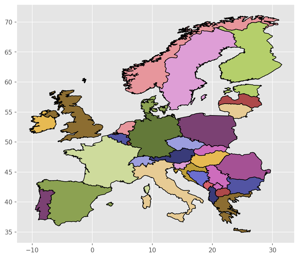
resources/offshore_shapes.geojson: EEZ shapes out of country selection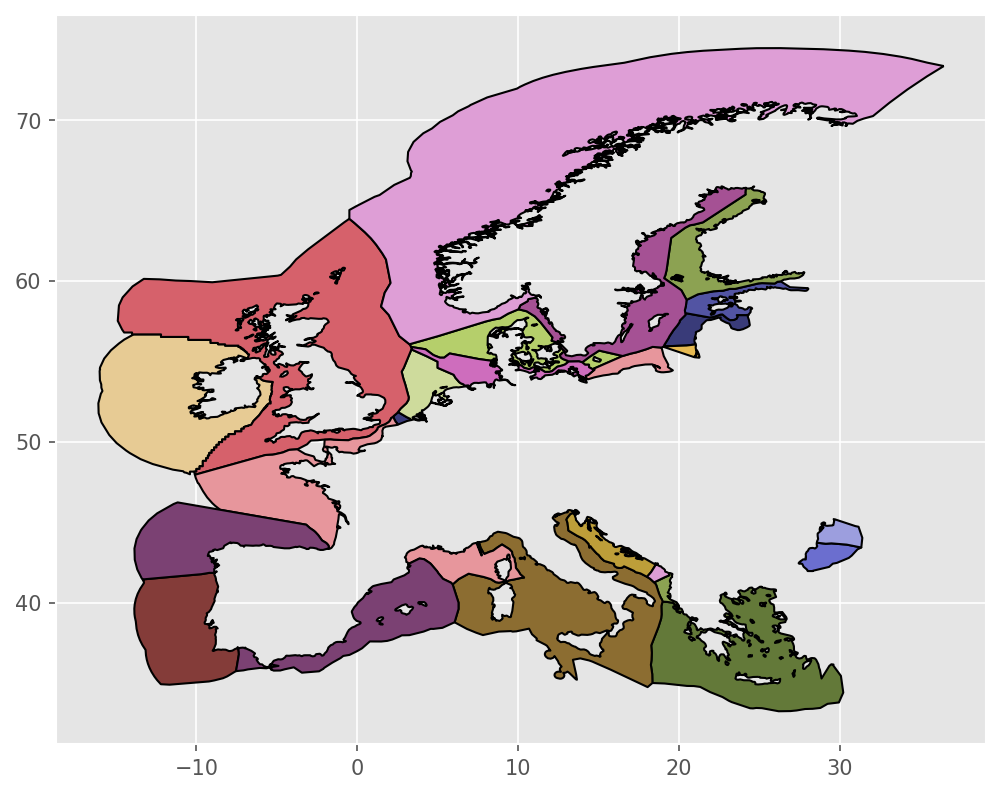
resources/europe_shape.geojson: Shape of Europe including countries and EEZ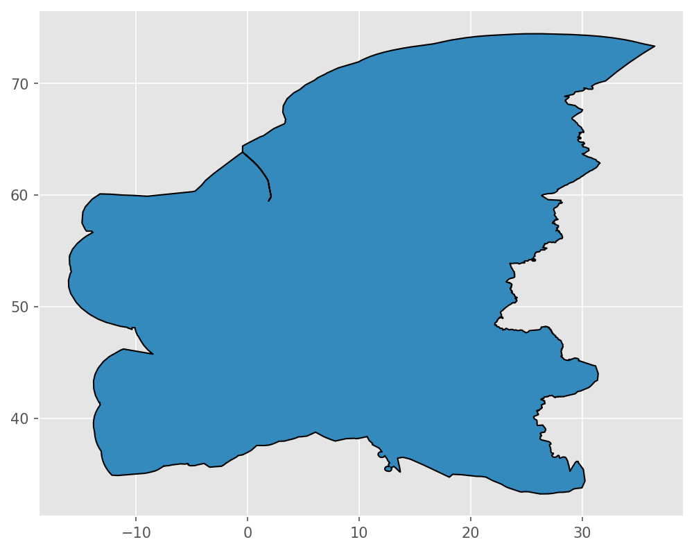
resources/nuts3_shapes.geojson: NUTS3 shapes out of country selection including population and GDP data.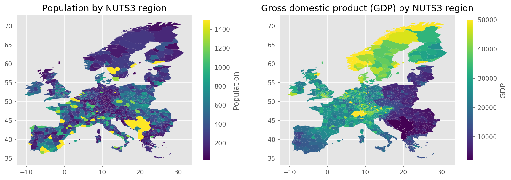
Description#
Rule build_powerplants#
Retrieves conventional powerplant capacities and locations from
powerplantmatching, assigns
these to buses and creates a .csv file. It is possible to amend the
powerplant database with custom entries provided in
data/custom_powerplants.csv.
Lastly, for every substation, powerplants with zero-initial capacity can be added for certain fuel types automatically.
Relevant Settings#
electricity:
  powerplants_filter:
  custom_powerplants:
  everywhere_powerplants:
See also
Documentation of the configuration file config/config.yaml at
Rule add_electricity
Inputs#
networks/base.nc: confer Rule base_network.data/custom_powerplants.csv: custom powerplants in the same format as powerplantmatching provides
Outputs#
resource/powerplants.csv: A list of conventional power plants (i.e. neither wind nor solar) with fields for name, fuel type, technology, country, capacity in MW, duration, commissioning year, retrofit year, latitude, longitude, and dam information as documented in the powerplantmatching README; additionally it includes information on the closest substation/bus innetworks/base.nc.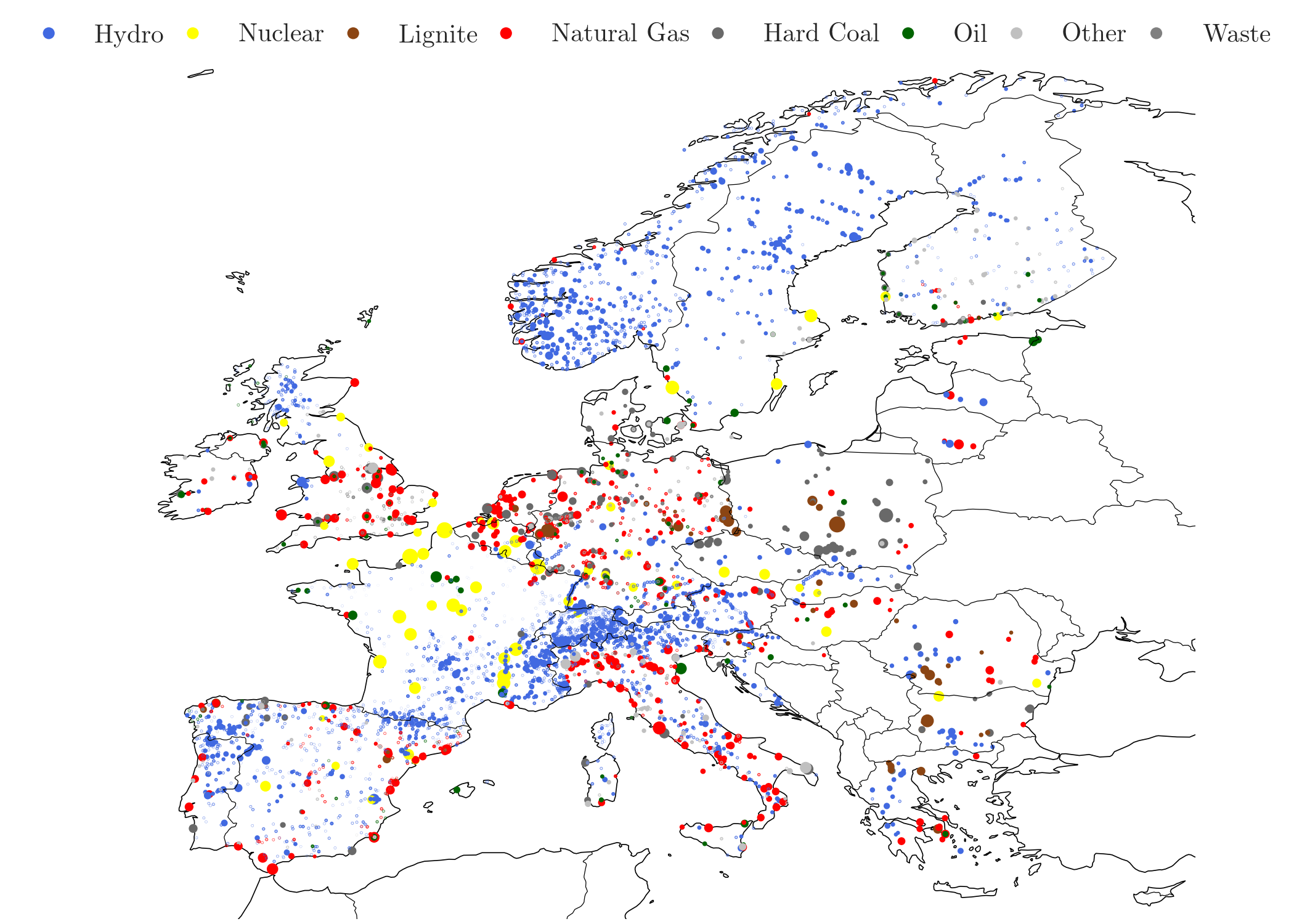
Source: powerplantmatching on GitHub
Description#
The configuration options electricity: powerplants_filter and electricity: custom_powerplants can be used to control whether data should be retrieved from the original powerplants database or from custom amendmends. These specify pandas.query commands.
In addition the configuration option electricity: everywhere_powerplants can be used to place powerplants with zero-initial capacity of certain fuel types at all substations.
Adding all powerplants from custom:
powerplants_filter: false
custom_powerplants: true
Replacing powerplants in e.g. Germany by custom data:
powerplants_filter: Country not in ['Germany']
custom_powerplants: true
or
powerplants_filter: Country not in ['Germany']
custom_powerplants: Country in ['Germany']
Adding additional built year constraints:
powerplants_filter: Country not in ['Germany'] and YearCommissioned <= 2015
custom_powerplants: YearCommissioned <= 2015
Adding powerplants at all substations for 4 conventional carrier types:
everywhere_powerplants: ['Natural Gas', 'Coal', 'nuclear', 'OCGT']
Rule build_electricity_demand#
This rule downloads the load data from Open Power System Data Time series. For all countries in
the network, the per country load timeseries are extracted from the dataset.
After filling small gaps linearly and large gaps by copying time-slice of a
given period, the load data is exported to a .csv file.
Relevant Settings#
snapshots:

load:
    interpolate_limit: time_shift_for_large_gaps: manual_adjustments:
See also
Documentation of the configuration file config/config.yaml at
load
Inputs#
data/electricity_demand_raw.csv:
Outputs#
resources/electricity_demand.csv:
Rule build_monthly_prices#
This script extracts monthly fuel prices of oil, gas, coal and lignite, as well as CO2 prices.
Inputs#
data/energy-price-trends-xlsx-5619002.xlsx: energy price index of fossil fuelsemission-spot-primary-market-auction-report-2019-data.xls: CO2 Prices spot primary auction
Outputs#
data/validation/monthly_fuel_price.csvdata/validation/CO2_price_2019.csv
Description#
The rule build_monthly_prices collects monthly fuel prices and CO2 prices
and translates them from different input sources to pypsa syntax
- Data sources:
[1] Fuel price index. Destatis https://www.destatis.de/EN/Home/_node.html [2] average annual fuel price lignite, ENTSO-E https://2020.entsos-tyndp-scenarios.eu/fuel-commodities-and-carbon-prices/ [3] CO2 Prices, Emission spot primary auction, EEX https://www.eex.com/en/market-data/environmental-markets/eua-primary-auction-spot-download
Data was accessed at 16.5.2023
Rule build_ship_raster#
Transforms the global ship density data from the `World Bank Data Catalogue.
<https://datacatalog.worldbank.org/search/dataset/0037580/Global-Shipping-Traffic-Density>`_ to the size of the considered cutout. The global ship density raster is later used for the exclusion when calculating the offshore potentials.
Relevant Settings#
renewable:
    {technology}:
        cutout:
See also
Documentation of the configuration file config/config.yaml at
renewable
Inputs#
data/bundle/shipdensity/shipdensity_global.zip: Global shipping traffic density from World Bank Data Catalogue.
Outputs#
resources/europe_shipdensity_raster.nc: Reduced version of global shipping traffic density from World Bank Data Catalogue to reduce computation time.
Description#
Rule determine_availability_matrix_MD_UA#
Create land elibility analysis for Ukraine and Moldova with different datasets.
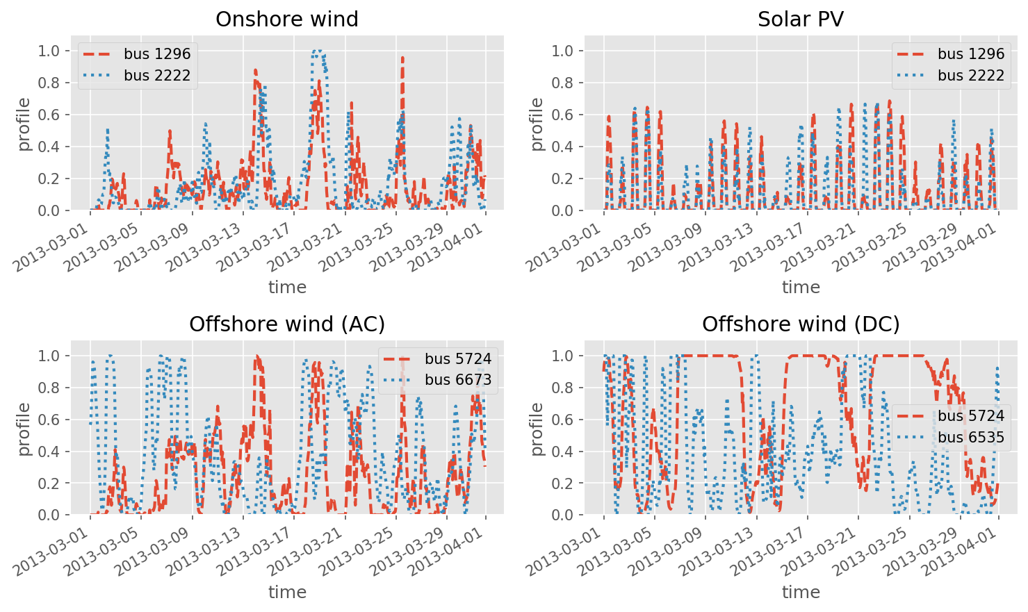
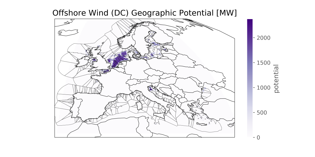
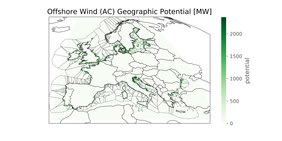
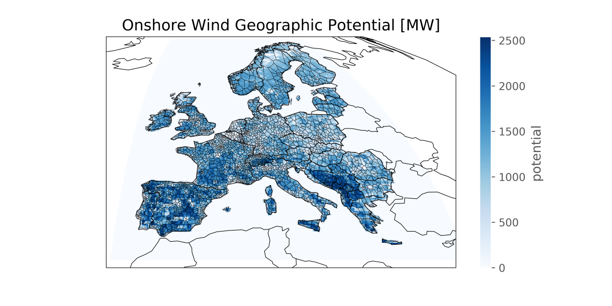
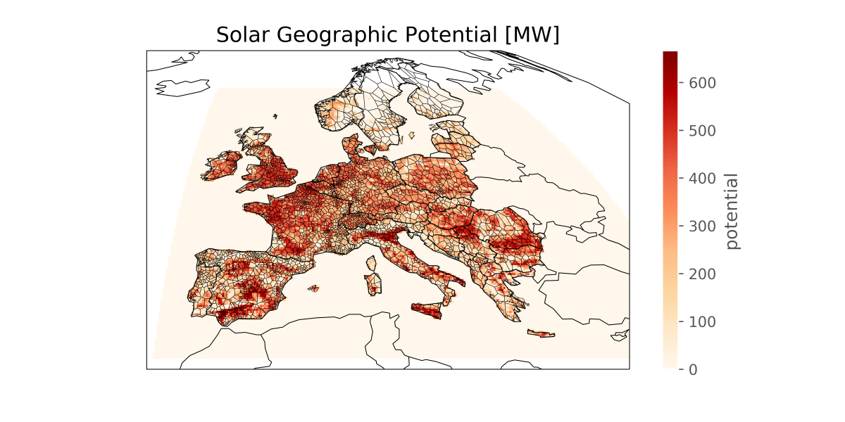
Rule build_renewable_profiles#
Calculates for each network node the (i) installable capacity (based on land- use), (ii) the available generation time series (based on weather data), and (iii) the average distance from the node for onshore wind, AC-connected offshore wind, DC-connected offshore wind and solar PV generators. In addition for offshore wind it calculates the fraction of the grid connection which is under water.
Note
Hydroelectric profiles are built in script build_hydro_profiles.
Relevant settings#
snapshots:

atlite:
    nprocesses:

renewable:
    {technology}:
        cutout: corine: luisa: grid_codes: distance: natura: max_depth:
        max_shore_distance: min_shore_distance: capacity_per_sqkm:
        correction_factor: min_p_max_pu: clip_p_max_pu: resource:
Inputs#
data/bundle/corine/g250_clc06_V18_5.tif: CORINE Land Cover (CLC) inventory on 44 classes of land use (e.g. forests, arable land, industrial, urban areas) at 100m resolution.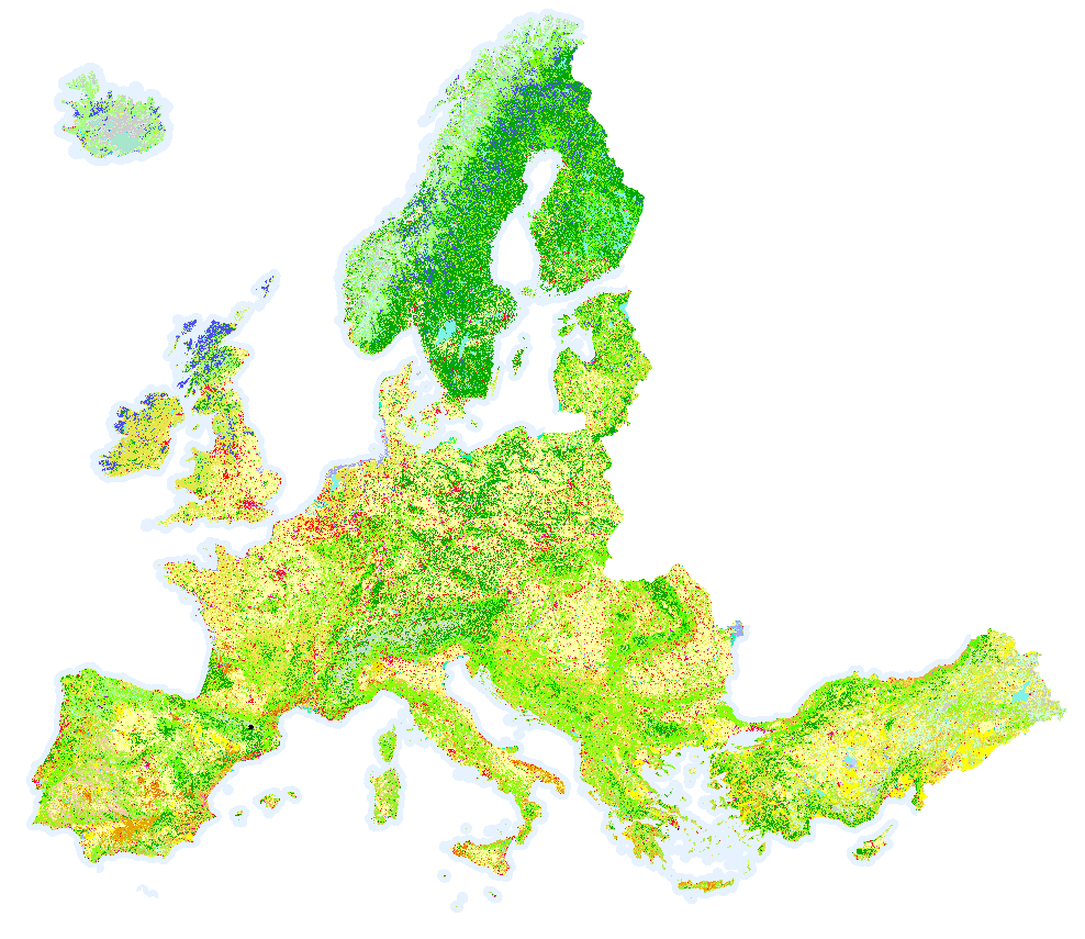
data/LUISA_basemap_020321_50m.tif: LUISA Base Map land coverage dataset at 50m resolution similar to CORINE. For codes in relation to CORINE land cover, see Annex 1 of the technical documentation.data/bundle/GEBCO_2014_2D.nc: A bathymetric data set with a global terrain model for ocean and land at 15 arc-second intervals by the General Bathymetric Chart of the Oceans (GEBCO).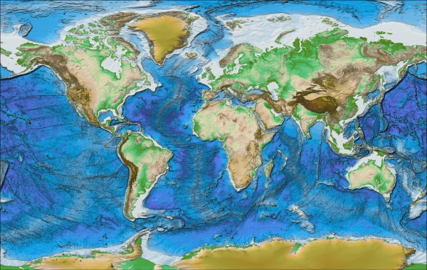
Source: GEBCO
resources/natura.tiff: confer Rule build_natura_rasterresources/offshore_shapes.geojson: confer Rule build_shapesresources/regions_onshore.geojson: (if not offshore wind), confer Rule build_bus_regionsresources/regions_offshore.geojson: (if offshore wind), Rule build_bus_regions"cutouts/" + params["renewable"][{technology}]['cutout']: Rule build_cutoutnetworks/base.nc: Rule base_network
Outputs#
resources/profile_{technology}.ncwith the following structureField
Dimensions
Description
profile
bus, time
the per unit hourly availability factors for each node
weight
bus
sum of the layout weighting for each node
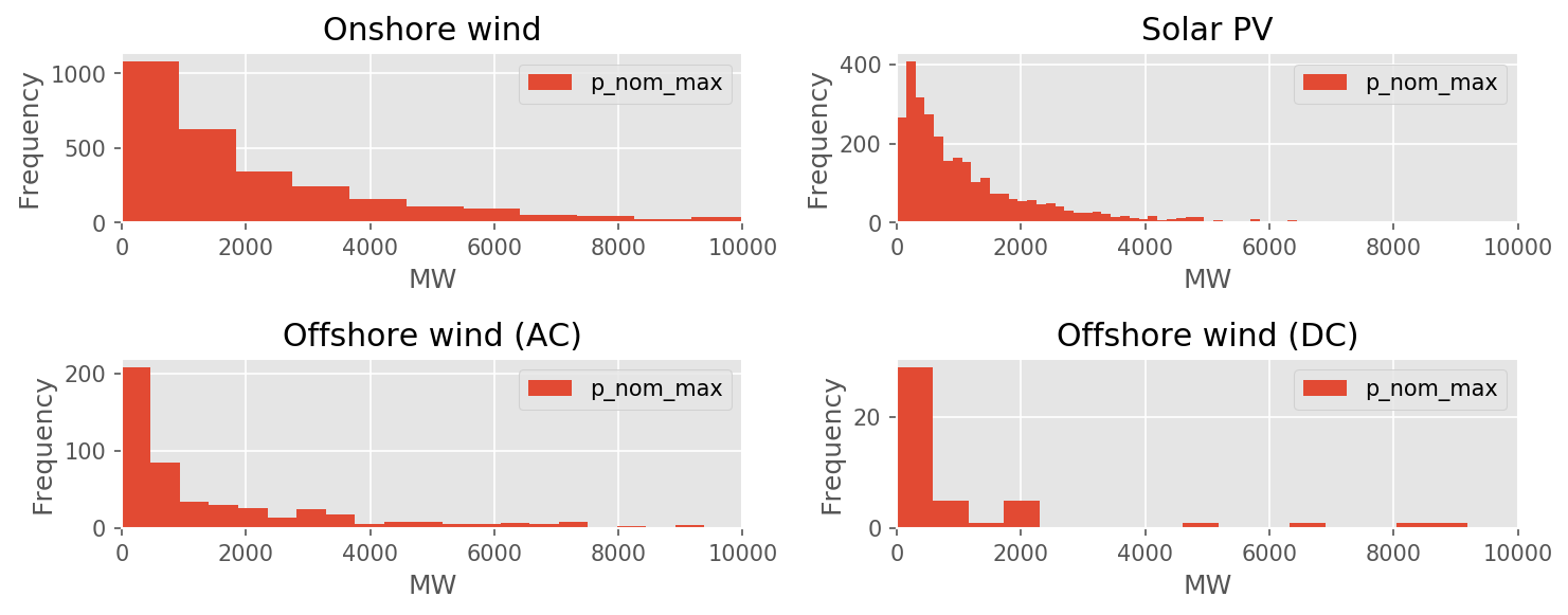
p_nom_max
bus
maximal installable capacity at the node (in MW)
potential
y, x
layout of generator units at cutout grid cells inside the Voronoi cell (maximal installable capacity at each grid cell multiplied by capacity factor)
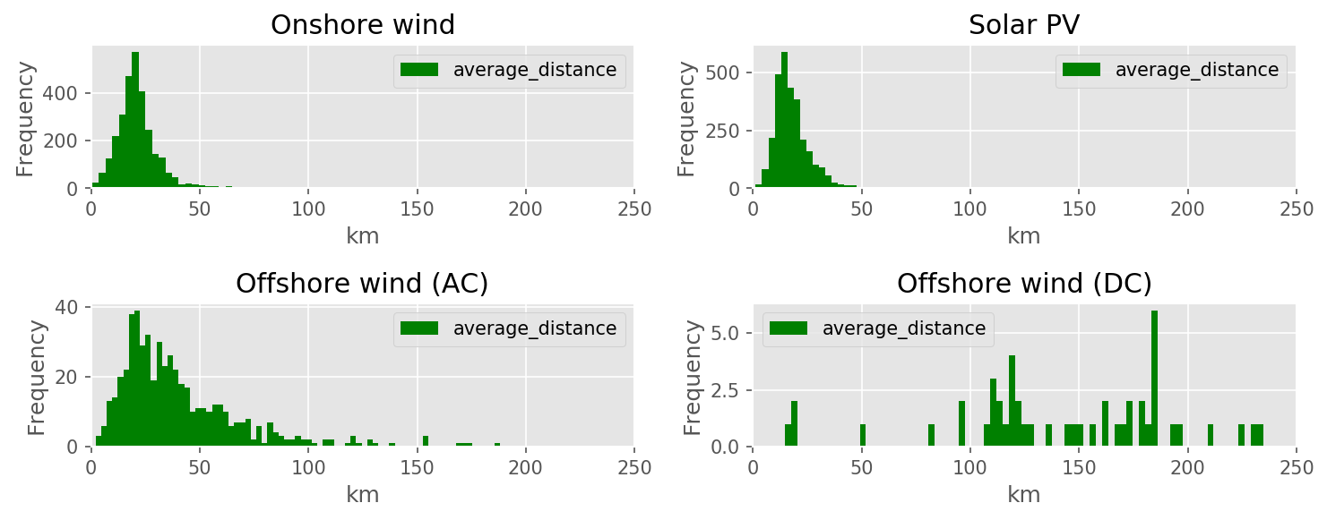
average_distance
bus
average distance of units in the Voronoi cell to the grid node (in km)
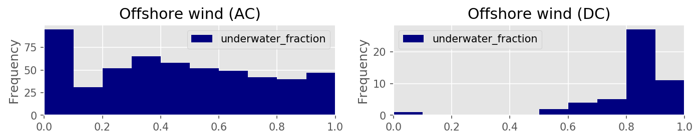
underwater_fraction
bus
fraction of the average connection distance which is under water (only for offshore)
profile
p_nom_max
potential

average_distance
underwater_fraction
Description#
This script functions at two main spatial resolutions: the resolution of the network nodes and their Voronoi cells, and the resolution of the cutout grid cells for the weather data. Typically the weather data grid is finer than the network nodes, so we have to work out the distribution of generators across the grid cells within each Voronoi cell. This is done by taking account of a combination of the available land at each grid cell and the capacity factor there.
First the script computes how much of the technology can be installed at each cutout grid cell and each node using the atlite library. This uses the CORINE land use data, LUISA land use data, Natura2000 nature reserves, GEBCO bathymetry data, and shipping lanes.
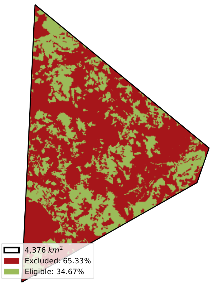
To compute the layout of generators in each node’s Voronoi cell, the installable potential in each grid cell is multiplied with the capacity factor at each grid cell. This is done since we assume more generators are installed at cells with a higher capacity factor.
This layout is then used to compute the generation availability time series from
the weather data cutout from atlite.
The maximal installable potential for the node (p_nom_max) is computed by adding up the installable potentials of the individual grid cells. If the model comes close to this limit, then the time series may slightly overestimate production since it is assumed the geographical distribution is proportional to capacity factor.
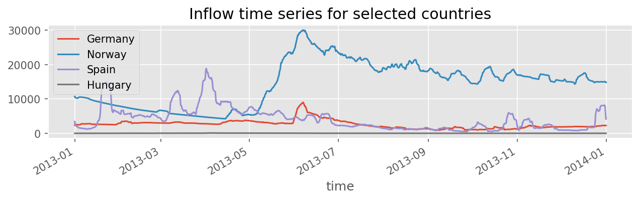
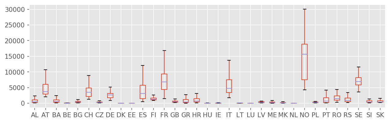
Rule build_hydro_profile#
Build hydroelectric inflow time-series for each country.
Relevant Settings#
countries:

renewable:
    hydro:
        cutout:
        clip_min_inflow:
See also
Documentation of the configuration file config/config.yaml at
Top-level configuration, renewable
Inputs#
data/bundle/eia_hydro_annual_generation.csv: Hydroelectricity net generation per country and year (EIA)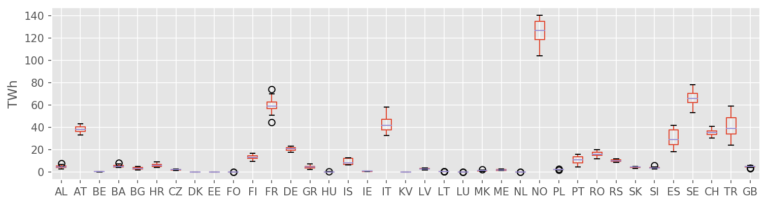
resources/country_shapes.geojson: confer Rule build_shapes"cutouts/" + config["renewable"]['hydro']['cutout']: confer Rule build_cutout
Outputs#
resources/profile_hydro.nc:Field
Dimensions
Description
inflow
countries, time
Inflow to the state of charge (in MW), e.g. due to river inflow in hydro reservoir.
Description#
See also
Rule add_electricity#
Adds electrical generators and existing hydro storage units to a base network.
Relevant Settings#
costs:
    year:
    version:
    dicountrate:
    emission_prices:

electricity:
    max_hours:
    marginal_cost:
    capital_cost:
    conventional_carriers:
    co2limit:
    extendable_carriers:
    estimate_renewable_capacities:


load:
    scaling_factor:

renewable:
    hydro:
        carriers:
        hydro_max_hours:
        hydro_capital_cost:

lines:
    length_factor:
See also
Documentation of the configuration file config/config.yaml at costs,
electricity, load, renewable, conventional
Inputs#
resources/costs.csv: The database of cost assumptions for all included technologies for specific years from various sources; e.g. discount rate, lifetime, investment (CAPEX), fixed operation and maintenance (FOM), variable operation and maintenance (VOM), fuel costs, efficiency, carbon-dioxide intensity.data/bundle/hydro_capacities.csv: Hydropower plant store/discharge power capacities, energy storage capacity, and average hourly inflow by country.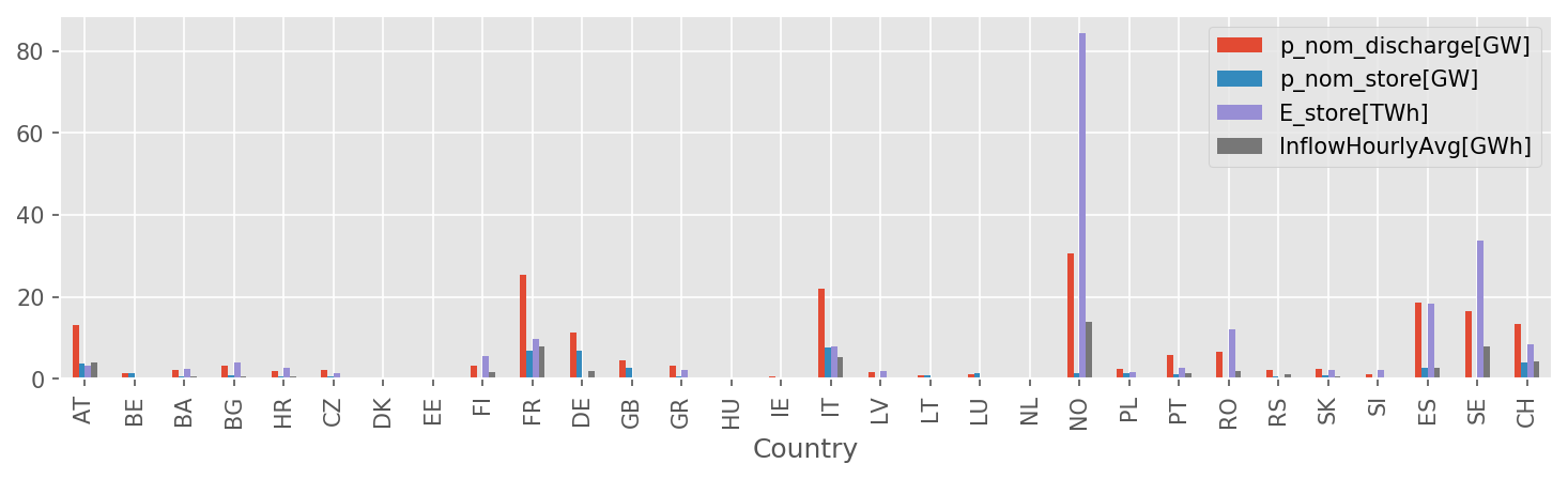
data/geth2015_hydro_capacities.csv: alternative to capacities above; not currently used!resources/electricity_demand.csvHourly per-country electricity demand profiles.resources/regions_onshore.geojson: confer Rule build_bus_regionsresources/nuts3_shapes.geojson: confer Rule build_shapesresources/powerplants.csv: confer Rule build_powerplantsresources/profile_{}.nc: all technologies inconfig["renewables"].keys(), confer Rule build_renewable_profiles.networks/base.nc: confer Rule base_network
Outputs#
networks/elec.nc: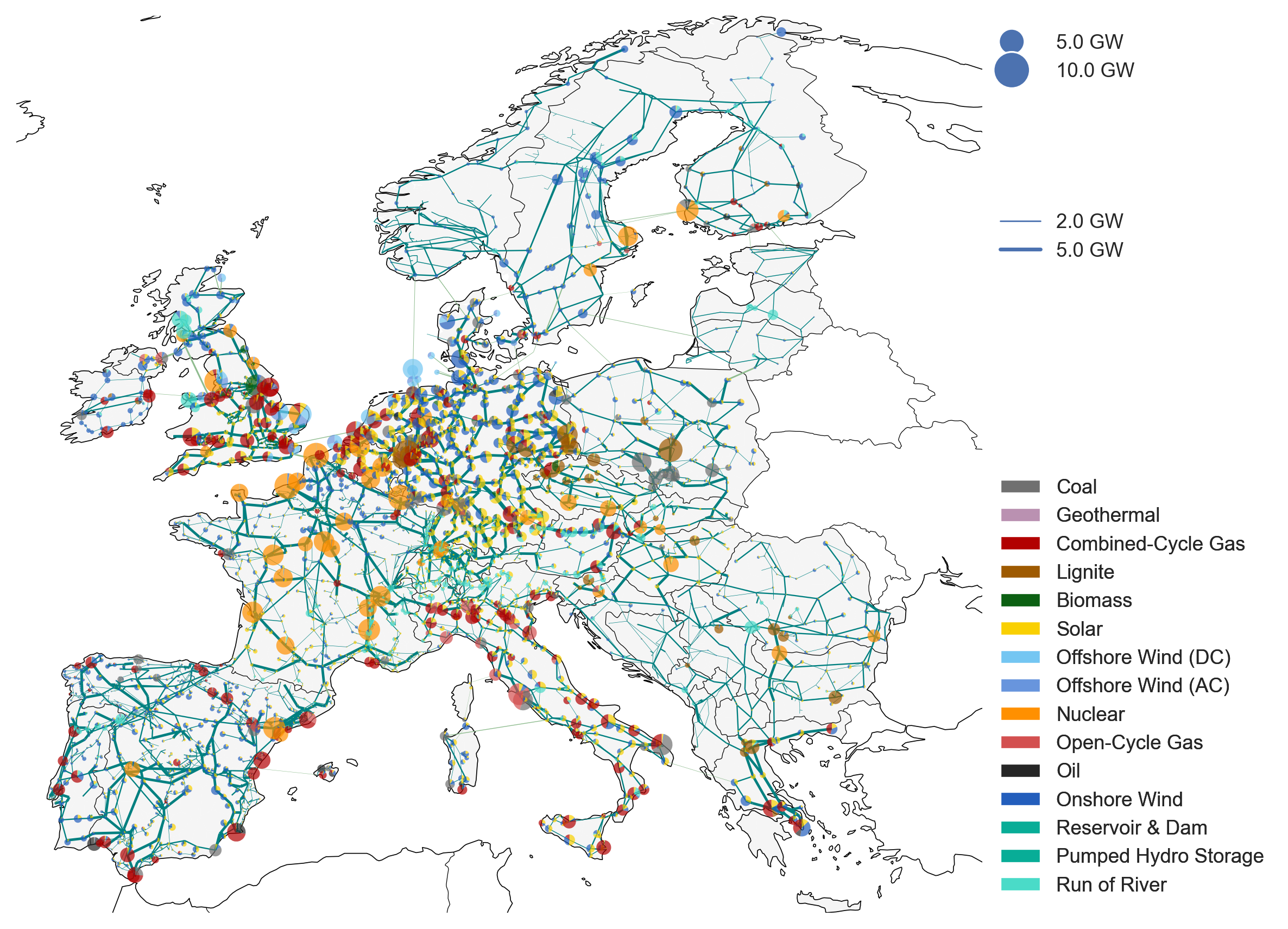
Description#
The rule add_electricity ties all the different data inputs from the preceding rules together into a detailed PyPSA network that is stored in networks/elec.nc. It includes:
today’s transmission topology and transfer capacities (optionally including lines which are under construction according to the config settings
lines: under_constructionandlinks: under_construction),today’s thermal and hydro power generation capacities (for the technologies listed in the config setting
electricity: conventional_carriers), andtoday’s load time-series (upsampled in a top-down approach according to population and gross domestic product)
It further adds extendable generators with zero capacity for
photovoltaic, onshore and AC- as well as DC-connected offshore wind installations with today’s locational, hourly wind and solar capacity factors (but no current capacities),
additional open- and combined-cycle gas turbines (if
OCGTand/orCCGTis listed in the config settingelectricity: extendable_carriers)